
This report was produced by the following authors (affiliations given as of the time of the competition, 2023):
- LDBC: Gábor Szárnyas, David Püroja
- Alibaba: Xiaojian Luo, Ke Meng, Wenyuan Yu
- Ant Group: Likang Chen, Heng Lin, Shipeng Qi
- Intel: Sriram Aananthakrishnan, Pascal Costanza, Henry A. Gabb, Yves Vandriessche
Introduction
Graph analytics and why it matters
Over the last few years, Gartner has consistently ranked graph analytics, graph processing, knowledge graphs, and context-enriched analysis (e.g. graph neural networks) among its top data science trends. This is because connected data, or graphs, are everywhere. Biochemical pathways, electrical grids, roadmaps, and communications networks are common examples of graphs. Because graphs are everywhere, it stands to reason that graph processing is also everywhere. Operations on such connected data invoke various graph analytics algorithms to extract useful information embedded in the connections. For example, web searches examine the connections among webpages to find the most relevant information. Social networks use friend connections to identify communities of people with similar interests. Mapping software looks for optimal routes in road networks.
Similarly, the graphs themselves are highly varied. Some are large and some are small. Some are relatively dense while others are very sparse. Some graphs have highly-skewed degree distributions. For example, the X (formerly Twitter) network is skewed because some people have millions of followers while most have only a few. Web graphs, on the other hand, tend to have a high average degree. Road networks often have a high diameter (the length of the path between the most distant nodes). All of these characteristics affect the performance of graph algorithms.
The computational landscape of graph analytics is very diverse, so no single graph and algorithm pair can represent the entire computational space. Several combinations are needed to give a comprehensive, objective, and reproducible representation of graph analytics performance because optimizations that work well for one graph topology might not work well for others.
GAPBS vs. Graphalytics
Good benchmarks are available to measure the performance of graph analytics software and hardware. The GAP Benchmark Suite from the University of California, Berkeley runs six common algorithms on five graphs with different characteristics to give good coverage of the graph analytics landscape (Beamer et al., 2015). Another advantage is that GAP is easy to run, so it was chosen for a recent comparison of several academic software packages for graph analysis (Azad et al., 2020). However, it does not have automatic correctness checking and its graphs are fixed-size and small by modern standards.
LDBC Graphalytics is more of an industrial-strength benchmark consisting of “six deterministic algorithms, standard datasets, synthetic dataset generators, and reference output, that enable objective comparison of graph analysis platforms” (Iosup et al., 2016). It is not as easy to run as GAP, but it covers similar regions of the graph analytics landscape and offers a few key advantages. First, it is strictly deterministic and provides reference output to make correctness checking easier. Second, its input graphs are classified by size, some of which are considerably larger than those provided by GAP. Third, the Graphalytics specification is maintained and updated by the LDBC. In 2023, the LDBC sponsored an open competition for graph practitioners to compare their hardware and/or software using Graphalytics. The results of this competition are described in the next section.
It is worth noting that both GAP and Graphalytics measure static graph analytics. SAGA-Bench is a better option for use-cases that require streaming graphs (Basak et al., 2020).
LDBC Graphalytics 2023 Competition
In 2023, we ran a competition on all Graphalytics algorithms (BFS, CDLP, LCC, PR, SSSP, WCC) and datasets of all sizes (S, M, L, XL, 2XL, 3XL). We received five submissions from three different vendors.
Submissions
First, we provide a brief description of each team’s hardware and software environments.
Ant Group submissions
The Ant Group team ran a Graphalytics implementation on the GeaCompute data processing platform. The benchmark was run on a cluster of ecs.c8i.24xlarge and ecs.c8a.48xlarge cloud instances:
- Each ecs.c8i.24xlarge cloud instance has a 96-core Intel Xeon Platinum 8475B with 192 GB of main memory and 8 TB external storage on Alibaba Cloud Capacity NAS.
- Each ecs.c8a.48xlarge cloud instance has a 192-core AMD EPYC Genoa 9T24 with 384 GB of main memory and 8 TB external storage on Alibaba Cloud Capacity NAS.
The benchmark used different numbers of instances for different scale data. For S-scale, M-scale, L-scale, XL-scale data, 1, 2, 4, 16 instances were used. For 2XL and 3XL scales, 24 instances were used. The three-year total costs of ownership are the following:
- 1 instance: 217,609.99 USD,
- 2 instances: 309,472.61 USD,
- 4 instances: 457,058.18 USD,
- 16 instances: 1,548,135.04 USD,
- 24 instances: 2,204,702.88 USD.
Alibaba submission
The Alibaba team ran a Graphalytics implementation on the libgrape-lite library. It has Graphalytics implementations for both GPU and CPU versions, so they submitted execution time results on both types of hardware.
-
The GPU version ran on a single ebmgn7e.32xlarge cloud instance. The instance features two Intel(R) Xeon(R) Platinum 8396 @ 2.70 GHz CPUs, each with 32 cores. It has 1 TB of main memory and is equipped with 8 Nvidia A100 GPUs. The external storage used is ESSD PL1, and the operating system is Ubuntu 20.04.5 LTS. The total cost of ownership for three years for this version was 456,697.00 USD.
-
The CPU version ran on a cluster of r7.16xlarge cloud instances. For S-scale data, 2 instances were used; for M-scale, 4 instances; and for L, XL, 2XL and 3XL scales, 8 instances were used. Each cloud instance has a 32-core Intel(R) Xeon(R) Platinum 8480B CPU, with 512 GB of main memory. The external storage used is Alibaba Cloud Capacity NAS, and the operating system is Ubuntu 20.04.5 LTS. The three-year total costs of ownership for these configurations were the following:
- 2 instances: 72,328.41 USD,
- 4 instances: 114,656.82 USD,
- 8 instances: 199,308.88 USD.
Intel submissions
The Intel team ran the unmodified GraphBLAS reference implementation of Graphalytics. The benchmark was run on on-premises servers:
- A custom server with a two-socket Intel Xeon Platinum 8480 (224 hardware threads) with 1 TB 4800 MHz DDR5 RDIMM RAM and 7.6 TB Solidigm D7-P5510 NVMe. The operating system was Ubuntu 22.04.2 LTS. The three-year total cost of ownership was calculated based on public vendor purchase prices for an equivalent system, resulting in 51,826 USD.
- For dataset sizes S to L, a PowerEdge R650 server with an Intel Xeon Gold 6342, 16 GB DDR4 RDIMM RAM, and 960 GB SSD, running Ubuntu 22.04. The three-year total cost of ownership was 15,354.81 USD.
Benchmark phases
The Graphalytics benchmark’s workload includes the following phases:
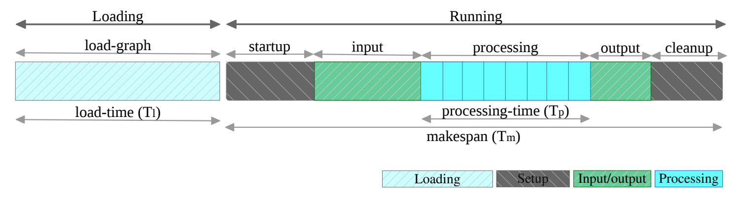
The key performance metrics used in the competition are the following:
- Makespan (in seconds): The time between the Graphalytics driver issuing the command to execute an algorithm on a (previously uploaded) graph and the output of the algorithm being made available to the driver. The makespan can be further divided into processing time and overhead. The makespan metric corresponds to the operation of a cold graph-processing system, which depicts the situation where the system is started up, processes a single dataset using a single algorithm, and then is shut down.
- Processing time (in seconds): The time required to execute an actual algorithm. This does not include platform-specific overhead, such as allocating resources, loading the graph from the file system, or graph partitioning. The processing time metric corresponds to the operation of an in-production, warmed-up graph-processing system, where especially loading of the graph from the file system and graph partitioning, both of which are typically done only once and are algorithm-independent, are not considered.
Benchmark results and analysis
The following tables show the results per dataset size, first ranked by price-adjusted processing throughput then by absolute makespan time.
Price-adjusted throughput and pricing results
Legend for the table header:
MS thru./$: Price-adjusted makespan throughput (per USD).Proc. thru./$: Price-adjusted processing throughput (per USD). By default, the results are sorted on this column (descending) per dataset size.Pricing ($): Total cost of ownership in USD.
| # | Size | Platform | Environment | MS thru./$ | Proc. thru./$ | Pricing ($) |
|---|---|---|---|---|---|---|
| 1. | S | libgrape-gpu | ebmgn7e.32xlarge | 0.080 | 58.349 | 456,697.00 |
| 2. | S | libgrape-lite | r7.16xlarge | 1.454 | 37.403 | 72,328.41 |
| 3. | S | GraphBLAS | bare metal, Xeon Gold 6342 |
3.051 | 11.452 | 15,354.81 |
| 4. | S | GraphBLAS | bare metal, Xeon Platinum 8480 |
6.262 | 17.988 | 51,826.00 |
| 5. | S | GeaCompute | ecs.c8i.24xlarge / ecs.c8a.48xlarge | 7.838 | 15.727 | 217,609.99 |
| 1. | M | libgrape-gpu | ebmgn7e.32xlarge | 0.025 | 37.132 | 456,697.00 |
| 2. | M | libgrape-lite | r7.16xlarge | 0.492 | 25.441 | 114,656.82 |
| 3. | M | GraphBLAS | bare metal, Xeon Gold 6342 |
1.120 | 5.737 | 15,354.81 |
| 4. | M | GeaCompute | ecs.c8i.24xlarge / ecs.c8a.48xlarge | 1.938 | 5.880 | 309,472.61 |
| 5. | M | GraphBLAS | bare metal, Xeon Platinum 8480 |
2.658 | 5.319 | 51,826.00 |
| 1. | L | libgrape-gpu | ebmgn7e.32xlarge | 0.033 | 16.575 | 456,697.00 |
| 2. | L | libgrape-lite | r7.16xlarge | 0.145 | 8.987 | 199,308.88 |
| 3. | L | GeaCompute | ecs.c8i.24xlarge / ecs.c8a.48xlarge | 0.428 | 2.275 | 457,058.18 |
| 4. | L | GraphBLAS | bare metal, Xeon Gold 6342 |
0.621 | 2.131 | 15,354.81 |
| 5. | L | GraphBLAS | bare metal, Xeon Platinum 8480 |
0.923 | 1.945 | 51,826.00 |
| 1. | XL | libgrape-gpu | ebmgn7e.32xlarge | 0.015 | 3.981 | 456,697.00 |
| 2. | XL | libgrape-lite | r7.16xlarge | 0.065 | 2.072 | 199,308.88 |
| 3. | XL | GraphBLAS | bare metal, Xeon Platinum 8480 |
0.242 | 0.388 | 51,826.00 |
| 4. | XL | GeaCompute | ecs.c8i.24xlarge / ecs.c8a.48xlarge | 0.077 | 0.275 | 1,548,135.04 |
| 1. | 2XL | libgrape-gpu | ebmgn7e.32xlarge | 0.008 | 0.593 | 456,697.00 |
| 2. | 2XL | libgrape-lite | r7.16xlarge | 0.047 | 0.329 | 199,308.88 |
| 3. | 2XL | GeaCompute | ecs.c8i.24xlarge / ecs.c8a.48xlarge | 0.024 | 0.050 | 2,204,702.88 |
| 4. | 2XL | GraphBLAS | bare metal, Xeon Platinum 8480 |
0.034 | 0.039 | 51,826.00 |
| 1. | 3XL | libgrape-lite | r7.16xlarge | 0.013 | 0.066 | 199,308.88 |
| 2. | 3XL | GeaCompute | ecs.c8i.24xlarge / ecs.c8a.48xlarge | 0.005 | 0.008 | 2,204,702.88 |
Between sizes S and L, we can observe a clear pattern: GraphBLAS implementations have the lead on price-adjusted makespan throughput, while libgrape implementations rank higher on price-adjusted processing throughput, with libgrape-gpu dominating the price-adjusted processing throughput results, and GeaCompute taking the place in the middle. This trend largely continues for XL and 2XL datasets, for price-adjusted processing throughput, with libgrape-gpu leading followed by libgrape-lite, while for price-adjusted makespan throughput, GraphBLAS is best for XL and libgrape-lite wins for the 2XL size. On the 3XL datasets, the libgrape-lite implementation has an edge for price-adjusted results over GeaCompute.
Makespan and processing times
Legend for the table header:
Mean MS: Mean makespan (in seconds). By default, the results are sorted on these values (ascending) per dataset size.Mean proc. time: Mean processing time (in seconds).#Runs: The minimum number of runs conducted per entry.
| # | Size | Platform | Environment | Mean MS (s) | Mean proc. time (s) | #Runs |
|---|---|---|---|---|---|---|
| 1. | S | GeaCompute | ecs.c8i.24xlarge / ecs.c8a.48xlarge | 2.25 | 0.20 | 3 |
| 2. | S | GraphBLAS | bare metal, Xeon Platinum 8480 |
2.46 | 1.23 | 3 |
| 3. | S | libgrape-lite | r7.16xlarge | 9.51 | 0.37 | 3 |
| 4. | S | GraphBLAS | bare metal, Xeon Gold 6342 |
10.40 | 3.62 | 1 |
| 5. | S | libgrape-gpu | ebmgn7e.32xlarge | 27.42 | 0.04 | 3 |
| 1. | M | GeaCompute | ecs.c8i.24xlarge / ecs.c8a.48xlarge | 3.72 | 0.50 | 3 |
| 2. | M | GraphBLAS | bare metal, Xeon Platinum 8480 |
7.26 | 3.63 | 3 |
| 3. | M | libgrape-lite | r7.16xlarge | 17.73 | 0.34 | 3 |
| 4. | M | GraphBLAS | bare metal, Xeon Gold 6342 |
33.60 | 11.08 | 1 |
| 5. | M | libgrape-gpu | ebmgn7e.32xlarge | 85.91 | 0.06 | 3 |
| 1. | L | GeaCompute | ecs.c8i.24xlarge / ecs.c8a.48xlarge | 6.30 | 0.79 | 3 |
| 2. | L | GraphBLAS | bare metal, Xeon Platinum 8480 |
20.90 | 9.92 | 3 |
| 3. | L | libgrape-lite | r7.16xlarge | 34.65 | 0.56 | 3 |
| 4. | L | libgrape-gpu | ebmgn7e.32xlarge | 66.55 | 0.13 | 3 |
| 5. | L | GraphBLAS | bare metal, Xeon Gold 6342 |
104.82 | 30.56 | 1 |
| 1. | XL | GeaCompute | ecs.c8i.24xlarge / ecs.c8a.48xlarge | 11.83 | 2.31 | 3 |
| 2. | XL | libgrape-lite | r7.16xlarge | 77.63 | 2.42 | 3 |
| 3. | XL | GraphBLAS | bare metal, Xeon Platinum 8480 |
79.75 | 49.71 | 3 |
| 4. | XL | libgrape-gpu | ebmgn7e.32xlarge | 150.75 | 0.55 | 3 |
| 1. | 2XL | GeaCompute | ecs.c8i.24xlarge / ecs.c8a.48xlarge | 19.56 | 9.25 | 3 |
| 2. | 2XL | libgrape-lite | r7.16xlarge | 105.83 | 15.26 | 3 |
| 3. | 2XL | libgrape-gpu | ebmgn7e.32xlarge | 259.01 | 3.69 | 3 |
| 4. | 2XL | GraphBLAS | bare metal, Xeon Platinum 8480 |
570.77 | 492.87 | 3 |
| 1. | 3XL | GeaCompute | ecs.c8i.24xlarge / ecs.c8a.48xlarge | 90.17 | 60.39 | 3 |
| 2. | 3XL | libgrape-lite | r7.16xlarge | 383.52 | 75.48 | 3 |
Across all dataset sizes, GeaCompute consistently has the best mean makespan runtimes, i.e. it provides the best end-to-end runtimes. For mean processing times, the libgrape-gpu implementation has leads up to 2XL. The largest dataset size, 3XL, was only completed by two distributed implementations, libgrape-lite and GeaCompute, with GeaCompute producing better runtimes. GraphBLAS implementations have the slowest absolute runtimes.
Concluding remarks
This report presented the results of the Graphalytics Competition 2023. The results show a surprisingly large variance between end-to-end performance, processing time in a warmed-up state and total cost of ownership. GeaCompute won in the end-to-end category, the GPU-based libgrape-gpu library was the fastest in most cases for warmed-up processing, while GraphBLAS was the least expensive option.
We thank all participants who entered the competition in 2023. If you are interested in future iterations of the competition, please reach out to [email protected].
References
- Azad et al. (2020), Evaluation of Graph Analytics Frameworks Using the GAP Benchmark Suite, 2020 IEEE International Symposium on Workload Characterization (IISWC).
- Basak et al. (2020), SAGA-Bench: Software and Hardware Characterization of Streaming Graph Analytics Workloads, 2020 IEEE International Symposium on Performance Analysis of Systems and Software (ISPASS).
- Beamer et al. (2015), The GAP Benchmark Suite.
- Iosup et al. (2016), LDBC Graphalytics: A Benchmark for Large-Scale Graph Analysis on Parallel and Distributed Platforms, Proceedings of the VLDB Endowment, 9(13), 1317-1328.
- Mattson et al. (2013), Standards for Graph Algorithm Primitives, 2013 IEEE High Performance Extreme Computing Conference (HPEC).