PostgreSQL 19 Matched Graph Patterns without a Graph Engine. We Measured What That Cost

Guest blog post by Dmitriy Eremeev, Ivan Khramkov, Aleksey Teplov (T-Technologies, R&D Center).

Update, September 2026. Since we ran this, SQL/PGQ has been reverted from PostgreSQL and will not ship in version 19. The last pre-release to carry it is beta 3, which is what we measured. The numbers below are a record of a first attempt, not a guide to a shipping feature — but the part that matters most is about PostgreSQL’s planner rather than about the operator that was withdrawn, and that part still stands. The last section says which is which.

Graph-shaped questions turn up in ordinary applications all the time: who is connected to whom, which accounts share a device, what links this order to that supplier. The data is usually already in PostgreSQL, and answering those questions there has always meant spelling out one join per hop of the pattern, every time.

We work on graph analytics, so when a mainstream relational engine grows native pattern matching we want to know what it can actually do — not from the release notes, but from a benchmark designed to be hard. This is what we found.

What a graph pattern is

Suppose you have a Person table, a Person_knows_Person table linking one person to another, and a Country table. “Friends of friends who live in the same country as you” is a shape:

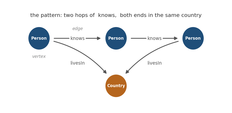
That picture is the whole vocabulary. The circles are vertices — rows in Person and Country. The arrows are edges — rows in Person_knows_Person, and the foreign key from a person to their country. One arrow traversed is a hop, and the whole shape is a pattern. Running the query means finding every set of rows arranged like the picture.

Real patterns get longer than this one, and they can loop back on themselves instead of running in a line.

In ordinary SQL you cannot write the shape; you write what it becomes. Each arrow is a join, each vertex a table to bring in, and the fact that both ends must land on the same country is a condition several lines away from the joins that produced them. The query works, but nothing in it looks like the picture, and adding one hop means editing it in three places.

The second way to write it

Until version 19 there was only one way in PostgreSQL, and it is the joins. SQL/PGQ provides the second: you declare a property graph — a statement, made once, that says which tables are vertices and which are edges — and then write the pattern itself. The operator is GRAPH_TABLE, and it hands the matches back as an ordinary relation that the rest of your query can join, filter and aggregate as usual. Other implementations exist — DuckPGQ over DuckDB, for one — and the version 19 betas were the first place it appeared in PostgreSQL.

The part that makes this worth measuring

PostgreSQL 19 did not gain a graph database. It gained a way of writing a query.

graph pattern → rewrite → ordinary relational plan → ordinary executor

There is no graph engine underneath, no graph storage, no graph-specific execution path. A property graph holds no data of its own; it is a declaration over tables that already exist. GRAPH_TABLE is handled in PostgreSQL’s rewriter, the same stage that expands views. The comment in the source says it plainly — “Convert GRAPH_TABLE clause into a subquery using relational operators” — and from there the ordinary planner and the ordinary executor do everything. You can read the code that does it — about 1 300 lines in rewriteGraphTable.c.

That is why this benchmark is interesting rather than routine. It is not a comparison between PostgreSQL and a graph database. It is a test of how far a mature relational optimiser gets on graph-shaped work when the pattern arrives in a nicer notation. Every result below, good or bad, belongs to that optimiser rather than to some new subsystem.

So we pointed LSQB at it, and wrote every one of its nine queries twice: once as a graph pattern, once as explicit joins.

Then we varied two things. Six graph sizes, from a few hundred megabytes to 650 million edges, all on one machine with one timeout. A seventh and much larger dataset, 2.1 billion edges, was run separately on bigger hardware and a longer limit; it is not part of the controlled series and never enters a comparison against the joins. And three ways of storing the five relations the schema needs but the raw data does not ship — as plain tables, as views, or as materialised views. That gives:

9 queries × 6 sizes × 3 storage strategies = 162 cells per form, or 18 configurations of each query

Every cell was run five times, in both forms. All of it on the PostgreSQL 19 pre-releases — beta 1, beta 2 and beta 3 — since that is what existed when we ran it; the numbers below are beta 3 unless stated otherwise.

The short version: the implementation executed six of LSQB’s nine graph patterns, five of them at every dataset size we tried. That is the PostgreSQL 19 beta we tested, on a benchmark built to stress graph engines — and every count it returned was correct, within a small factor of the same query written as joins. The three it does not execute are the three the benchmark designed to need algorithms PostgreSQL implements for no query at all. If your patterns are not those, this is usable today.

What the nine queries actually ask

LSQB is deliberately narrow. Every query matches a labelled pattern in a social network — people, posts, comments, tags, the places and organisations attached to them — and counts the matches. No filtering, no ranking, no aggregation beyond count(*). That is on purpose: the benchmark is testing one thing, how well the engine handles the joins that pattern matching turns into.

The nine fall into three groups, and the grouping predicts almost everything that follows.

	Query	What it looks for
Chains and stars	Q1	a chain of seven hops, Country through to TagClass
	Q4	four edges meeting at one message
	Q5	two different tags on a message and a reply to it
The same, with optional and negative edges	Q7	Q4, with two of the edges optional
	Q8	Q5, but the reply must not carry the first tag
Cycles through knows	Q2	a comment replying to a post, whose two authors know each other
	Q3	three people who all know each other and share a country
	Q6	a friend of a friend — a different person — interested in some tag
	Q9	Q6, but the two people must not know each other

An “optional” edge is a left outer join; a “negative” edge is an anti-join — the pattern matches when that edge is absent. The benchmark’s paper draws all nine as diagrams, which is the quickest way to see the shapes Figure 3 of the LSQB paper.

The third group is the one that separates graph engines from relational ones, and it is where this story ends up.

What runs, and what it costs

Six of the nine queries complete somewhere in the matrix, and five of those complete everywhere in it. The five are Q1, Q4, Q5, Q7 and Q8, at every size in the controlled series under plain tables or materialised views. Five of the nine still return on the separate 2.1-billion-edge run, in a 252 GB database. We did not look for a size at which they stop. The sixth, Q2, is the awkward one: it completes at SF 1 and SF 3 and nowhere else. Every value either form returned matched LDBC’s published answers, all 438 of them, and we could check that twice over: against the benchmark’s expected-output.csv and against the match counts printed in the LSQB paper.

Where both forms finish, the explicit joins lead by 1.25× to 2.55× on the set each size has in common, or 1.85× to 2.90× on the fixed pair Q5 and Q7 that every size shares. That is a factor, not an order of magnitude, on a first implementation running on the relational engine the server already had.

One thing to hold onto before reading any latency number here: we compared two implementations, not two query languages. The relational queries are LSQB’s own reference implementations; the SQL/PGQ ones we wrote. A better graph formulation may exist that we did not find, and we have no way to bound how much of the gap that accounts for. The fine print at the end lists the other differences.

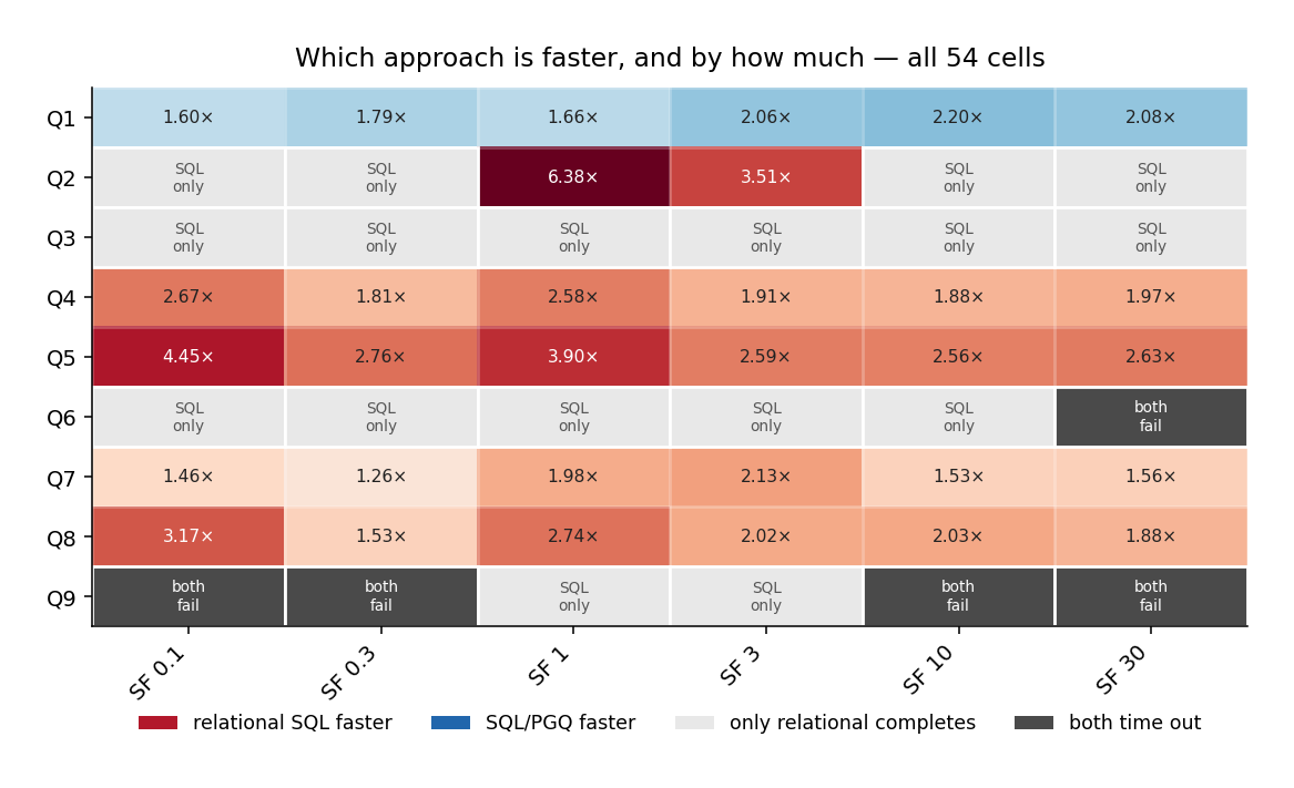
One blue row, five red, three grey. The grey rows are the queries where only the relational form finished at all.

Coverage, not latency, is where the work remains

The boundary is worth locating precisely, because it is mostly a property of specific patterns rather than of scale. Q3, Q6 and Q9 hit the ten-minute limit in all eighteen configurations, at every size from a few hundred megabytes upward, and Q2 returns at two sizes of six. Sixty-nine of the 162 query cells hit the limit, and they are concentrated in those four columns rather than spread across the matrix.

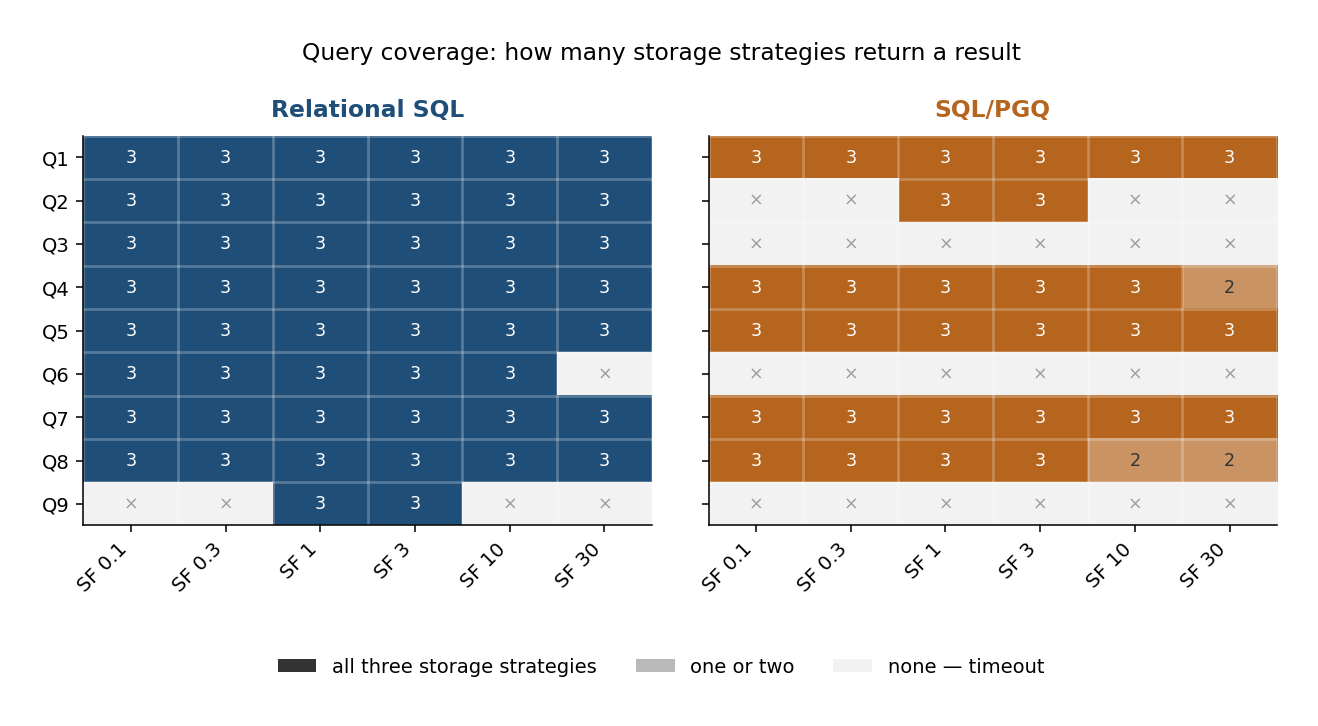
Three empty rows on the right, against two gaps on the left. Per query, out of its eighteen configurations:

Query	as a pattern	as explicit joins
Q1	18	18
Q2	6	18
Q3	0	18
Q4	17	18
Q5	18	18
Q6	0	15
Q7	18	18
Q8	16	18
Q9	0	6

Q3, Q6 and Q9 are exactly the three the benchmark’s authors single out as needing worst-case optimal joins or factorised processing. Both are ways of avoiding a fully materialised intermediate result when the final answer is much smaller than it. Q3 shows why that matters: at the smallest dataset it finds 30 456 triangles among 36 270 knows edges, but a planner that joins two tables at a time has to build every two-hop path before it can close the third edge — and there are necessarily far more two-hop paths than triangles, since most of them never close. The intermediate result is the problem, not the answer. PostgreSQL implements neither technique, for any query, graph-shaped or not. The coincidence is sharp enough to be worth taking seriously, though what the measurements establish is the coincidence rather than the cause. That the losses land precisely there, and nowhere else, is the useful part: the evidence points more strongly to a missing join strategy than to a fundamental problem in GRAPH_TABLE itself. The gap it leaves is wide. At that same smallest size the graph form does not answer Q3 in ten minutes, while the joins answer it in 1.459 seconds; Q6 has 55.6 million matches there and the join form counts them in three.

So the constraint to plan around is not that patterns are slower. It is that a few shapes do not run yet.

We were sure it was the statistics. It wasn’t — and that is useful

Our harness never ran ANALYZE. The planner was therefore sizing every step of every query from built-in defaults rather than from the data, and the obvious conclusion was that we had been measuring our own omission.

So we re-ran the entire matrix with ANALYZE first.

Not one query moved from timeout to completion. Five moved the other way. Four were one relational query that had been answering in about four seconds and now exceeds the ten-minute limit — at least 150 times worse, and the true factor is unknown because a cancelled query reports no duration. The plan says why: an anti-join estimated at one row against five million actual, feeding a nested loop over an unindexed table. Better statistics, worse plan.

That is one of the most useful things we learned, because it rules out the easy explanation. Whatever closes these queries, it is not missing statistics — which narrows the remaining work to cardinality estimation at the join and to the access paths available for it. Both are the kind of thing that improves release over release.

What the plans show

We captured a plan for every query in every configuration, in the same statistics state as the timings: 648 of them. GRAPH_TABLE is not a separate engine — it rewrites the pattern into ordinary SQL and hands it to the same planner. So we can read exactly what it produces.

It produces a bigger query. A SQL/PGQ plan reads a median of 2.2 times as many tables as the join form of the same question. Q6 relationally scans three; the graph form scans seven, three of them Person, because every edge in the pattern is joined back to the vertex tables its keys reference. The explicit form never needs that: it joins edge tables to one another directly.

That explains the direction of the latency gap. It does not explain the timeouts. On Q3 the query the rewrite produces is actually smaller than the join version, so something in plan selection defeats it, and we could not pin down what.

Where the pattern form wins

Q1 is faster under SQL/PGQ at every size we measured, by 1.60× to 2.20×. It has the longest chain and the most edges stored in their own tables, and that is the reason. The graph projection — the mapping that says which tables are vertices and which are edges — lets the planner walk narrow two-column edge tables instead of dragging the two largest relations in the schema along behind it.

That is worth more than one row of a table. It means the graph representation is not inherently the slower of the two. It wins where a pattern spans many separately stored edge relations, and loses where the relational form reaches an edge through a foreign-key column of a table it was going to read anyway. How you project the tables into a graph and which notation you write the query in are not independent choices, and on the right shape the newer one is already ahead.

The evidence is one query out of nine, so treat it as a hypothesis to test against your own workload rather than a rule. But it is the kind of result that says the remaining gap is in plan selection, not in the idea.

The regression that wasn’t a regression

In our first campaign, Q3 completed on beta 1: one configuration out of eighteen, 1.504 seconds, correct answer, while beta 2 and beta 3 both blew through 600 seconds. That is at least a 400-fold difference between consecutive pre-releases — at least, because a cancelled query reports no duration — and easily the most interesting number we had.

It did not survive the re-run. Under the controlled protocol that cell times out on beta 1 too, coverage becomes identical across all three versions query for query, and 160 of 162 plan combinations agree. So there was no regression. There was a planner, working without statistics, that happened to pick a workable plan once in eighteen tries — and we had reported it as a version difference because our protocol could not tell those two things apart.

The first campaign ran three repetitions in whatever order os.walk returned. That was enough to produce five cells where the arithmetic implied one repetition running 6 to 241 times slower than the rest, which looks a lot like planner instability and got a section of its own. Re-run with five repetitions in a fixed order, no cell spans more than a factor of 1.80. The bimodality was our query order: which queries had warmed the cache differed between configurations, and we had built a theory on top of it. There is now a control group that makes the point cleanly — five queries never touch the derived relations, so for two of the three storage strategies their SQL is identical and they must behave the same. Under the old protocol those pairs diverged by up to a factor of 18; under the new one they stay within 0.61–1.14.

If you take one thing from this post and it isn’t about SQL/PGQ, take that one.

Storage strategies: two of the three are interchangeable

The LSQB schema needs five relations the source data doesn’t provide, each a union over Comment and Post, and nothing in the standard says how to supply them. We tried all three ways.

Plain tables and materialised views performed similarly — 0.97× to 1.44× of each other, with no trend. Ordinary views were consistently worse, at 1.89× to 3.28×, for a mechanical reason: each of the five expands into a UNION ALL over two source tables, so a query touching four of them reaches the planner with eight scans where plain tables give four. They buy 38–42 % less disk, which one pass over the query set already outweighs.

If you are choosing: tables or materialised views, on whichever grounds suit your refresh story. The report has the full comparison, including load times and peak memory.

What the syntax does not take yet

Before any of the timing matters, some patterns cannot be written at all. Eight constructions are rejected, all of them during analysis rather than at run time, which at least means you find out immediately:

Rejected	Consequence
multiple path patterns in one GRAPH_TABLE clause	a pattern that is not a single walk must be split into several GRAPH_TABLE expressions by hand
element pattern quantifier is not supported	no variable-length paths, no transitive closure — see below
six more, including adjacent vertex patterns and non-local variable references	narrower ways of writing the same walk

The second is the one to check before planning anything. A quantifier is what lets you write “any number of hops” — the graph equivalent of asking for everyone reachable from Alice through knows, however many people are in the chain. Without it you can ask for friends, and friends of friends, and friends of friends of friends, but only by writing each length out as its own pattern. If your workload needs reachability, this release cannot express it.

All eight rejections come from parse_graphtable.c, and the full list with line numbers is in the report.

Should you use it?

Check the shape of your patterns first. In this benchmark one property turns out to be a surprisingly good predictor: the number of undirected knows edges a pattern matches separates completion from timeout exactly. The five patterns that match none complete in 16 to 18 of 18 configurations; the four that match one or more complete in 6 or 0. Nine queries is far too few to call that a rule, and knows is also the largest many-to-many relation in the schema, so the two explanations are not separated here. Still, it costs nothing to check against your own patterns before you commit to anything.

If your patterns look like Q1 — long chains over many separately stored edge types — SQL/PGQ in PostgreSQL 19 is already faster than the joins you would write out yourself. If they look like Q3, Q6 or Q9, we could not get the feature to complete them under any configuration we tested. For everything in between, budget a factor rather than an order of magnitude, and run plain EXPLAIN before running the query: both failure modes are visible in the plan without executing anything.

The fine print, which matters

As above: two implementations, not two query languages. Beyond the formulation, they read different physical layouts, one has primary keys and the other none, and knows is stored once in one and twice in the other. So the latency numbers compare our SQL/PGQ formulations against LSQB’s reference SQL — not the two languages in the abstract. That is the biggest threat to every figure above.

The server ran on packaged defaults throughout, shared_buffers at 128 MB and work_mem at 4 MB — an untuned baseline, not a production configuration. Every size shared one instance flavour, one timeout and one repetition count, so the series across sizes is controlled; only the SF 100 figures come from a different machine and a longer limit.

Where this leaves PostgreSQL 19

LSQB was written to separate graph workloads from relational ones — to be the benchmark graph engines pass and relational engines do not. A first implementation of a 2023 standard, measured on the PostgreSQL 19 betas and running on an unmodified relational planner, executes six of its nine patterns, five of them at every size in the controlled series. Every count it returned was correct, within a factor of the same query written as joins, and faster than that on the one pattern whose edges live in tables of their own rather than in foreign-key columns. That is a better starting position than the feature had any obligation to reach.

The three it does not execute are the three the benchmark associates with worst-case optimal joins or factorisation, which this engine implements for no query at all. On the evidence here that looks more like a gap in the optimiser than in the operator — the kind that closes release over release — though a formulation we did not try might yet shift the picture. Read as a drop-in replacement for a graph database on cyclic workloads, it is not ready, and we are not claiming it is.

For anyone weighing SQL/PGQ today: on the patterns it runs, it is already a shorter way to write a query that costs a factor. That is a trade a lot of workloads would take.

What the revert changes, and what it doesn’t

It is worth knowing why SQL/PGQ went, because the answer is not “it was slow”: the discussion turned on catalog and DDL behaviour — orphaned labels after cascade drops, pg_dump missing dependencies, rewrite paths reading table schemas without locks — none of which this benchmark exercises, and all 105 SQL/PGQ runs that returned a value — of 189 attempted — returned the published answer. So the numbers stand as measurements. What they no longer predict is latency or syntax, both of which belong to a rewriter that will be redesigned. What they do still give you is a baseline: Q3, Q6 and Q9 are the three the benchmark associates with worst-case optimal joins or factorisation, and the version we tested implements neither for any query at all — that is the planner, not the graph operator, and any new front end rewriting into ordinary relational plans would meet it in the same three places. Whether that boundary holds for whatever arrives next is a question for the next benchmark run — and a checkable one, since everything needed to re-run it is published. The report works through the split in full.

Everything is published

We wrote all of this up properly as a full disclosure report: every table, the captured plans, the threats to validity, and both measurement campaigns with their conditions stated side by side. It accompanies this post, and if you want the numbers rather than the narrative, that is where to find them.

The harness, schemas, query texts, raw results and all 648 plans are in the repository, each campaign alongside the version of the harness that produced it. If you re-run it and get something different, we would like to know.

This work was carried out by the T-Technologies, R&D Center team.